Behind the scenes: MICrONS video

Beyond eye candy: Anatomy of an advanced neuro visualization

This week I have the opportunity to publish one of my most challenging neuroscience visualization projects yet, and while it’s still fresh I’ve decided to show a little bit about my process and what goes on under the hood, from conception to delivery.

Neurons from a column of cortex. Their colors label their morphological types are a feature of their branching geometry. In this image they are not organized by their anatomical position, but instead using a low dimensional embedding (UMAP) of the multi-dimensional morphological measurements. Data from Schneider-Mizell et al 2025

Designing data visualization for video isn’t afforded the same luxuries of attention as for print or the web. A great scientific figure may have an extensive caption that is elaborated upon in the methods and results sections. There’s no time limit to how long someone can pour over it until it clicks. Similarly, a front-page Dataviz graphic can be prodded and scrutinized without limit, taking as much of the viewers time as they are willing to give it.

Video content on the other hand could be described as fast-facts, and has a different relationship to the attention economy. It often must fit a tiny allotted timeslot in film, or it must compete for attention in a stream of breaking news and new dance moves. If you don’t hook the viewer in the first few seconds, they’ll move onto the next one. While people can go back and re-watch the video as many times as they want, most of them won’t, so you only have a few seconds of attention span to deliver as big a punch as possible. So this article examines my process for taking primary research data and transforming it into engaging video segments, 1-2 minutes each.

As case study this post will break down the 5 short videos which each accompany one of the papers in the MICrONS Project collection. A couple of my renders were featured in the very accessible introduction Nature immersive article. The goal of this post is not to explain the contents of those papers, but to outline my creative process whereby I transform a curated selection of laboratory data into engaging motion graphic sequences. In each subsection I describe first in words what I wanted to convey, then show my initial storyboard sketch for that sequence, and the final video.

Background: It's important to mention that neurons in the Cerebral Cortex of the brain are organized into layers, each with different types of neurons which connect to each other in different ways. They are functionally organized into modular ‘Columns’ through all 6 layers. Check out A cubic Millimeter of Mouse Brain for a narrated visual primer on the layer and columns in the cortex, or The Neuron, the Synapse, and the Connectome for a more accessible introduction to the field of connectomics.

1. Functional connectomics spanning multiple areas of mouse visual cortex

Flagship paper / Technical:

The first video needed to introduce the scale and richness of the MICrONs cubic millimeter dataset; to convey what makes it unique and powerful. Key points are that it contains dense segmentations of ~100k neurons and half a billion synapses, within a cubic millimeter of visual cortex. Many of the neurons had been optically recorded with calcium imaging while the mouse was alive. A truly remarkable dataset: a completely reconstructed volume that spanned different brain regions, large enough to reconstruct complete dendritic branches, and a connectivity map between all the neurons at synaptic resolution.

This storyboard wasn’t strictly followed in the final version of the video. The scene was completely transformed over the course of the revision process, as the introduction it had to carry the most weight.

Video Description:
We open to a video from a functional 2-photon imaging plane acquired from this mouse — individual imaging planes play back real calcium imaging videos, with the functionally aligned neuron geometry coming into view before the densely segmented volume of the MICrONS cubic millimeter fades into view.

The camera then zooms in on a single synapse and orbits around the connection between the cells. A selection of firing neurons fade back into view, as the camera zooms back out, as the densely reconstructed layers of cortex fade into view. 4 example cells from different cortical layers are shown. Each is sequentially highlighted, followed by a collection of cells that are its synaptic partners, showing the richness of the dataset that combines both function and connectomic data in the same neurons.

2. Perisomatic ultrastructure efficiently classifies cells in mouse cortex

Classification: cell-type predictions across the volume.

How does a massive collection of cell geometry become a richly annotated dataset with cell-type information?
A column of cells through all the layers of cortex was manually annotated by experts, and used to train a model that could predict the cell types of the rest of the volume by only using the morphological characteristics of the cell nucleus, soma and peri-somatic areas.

A few snapshots from the preprint figures that I used to plan the scene. Wherever possible, I use the same color palette as the authors for visual consistency between the paper and the video, this was the video can be used as a reference.

I wanted to focus on the column (cylinder) with the various layer types, then focus on specifically the morphology of the soma and nucleus. Next we would morph into a low-dimensional representation to show the classification of ‘out of sample’ cells. Finally we would end on the cell types from the column being applied across the entire dataset.

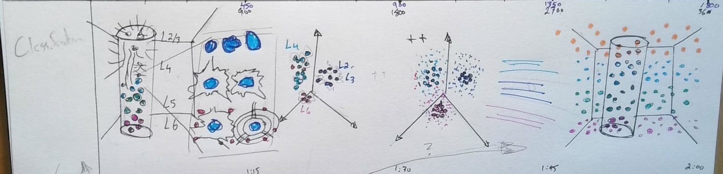
Video description:
We start by showing the entire volume of the cubic millimeter of visual cortex, without any color - indicating they are without any annotation. We then show examples of expert-annotated neurons from a column that spans all the cortical layers. The camera orbits this column of cells, and we are shown a smaller selection of cells. The soma and nuclei expand to show that the measurements come from these cell features. These expert annotated cells shift into a UMAP low-dimensional space, where expert-labeled cell types cluster by feature similarity, revealing the neurons grouped into cell type.

All remaining cells from the cubic millimeter fade into that same UMAP space, classified using the metamodel described in the paper. Layer-by-layer, reconstructed cells morph into their anatomical positions, showing how the metamodel predictions have provided cell type information for the entire MICrONS cubic millimeter dataset.

3. Inhibitory specificity from a connectomic census of mouse visual cortex

Layer-specific Morphology and Inhibitory Connectivity Patterns

Now considering the morphology of the dendritic branches, the neurons can be grouped together and categorized into their “Morphological Types”. They grouped the neurons this way and systematically analyzed the connectivity of all of the inhibitory cells input onto each different type of cell, to discover new inhibitory connectivity motifs.

For this video, the elements were taken from multiple figures from the article: The cortical column, a low dimensional representation, and the breakdown of synaptic connections onto each brain layer (Cell Cards).

Here the idea was to show the column neurons with their morphology, then to morph them into their low-dimensional embedding to explore their branching up close. We’d then introduce the inhibitory synaptic connectivity onto specific types, and cycle through the paper’s ‘Connectivity cards’ for each of the inhibitory neurons in the column.

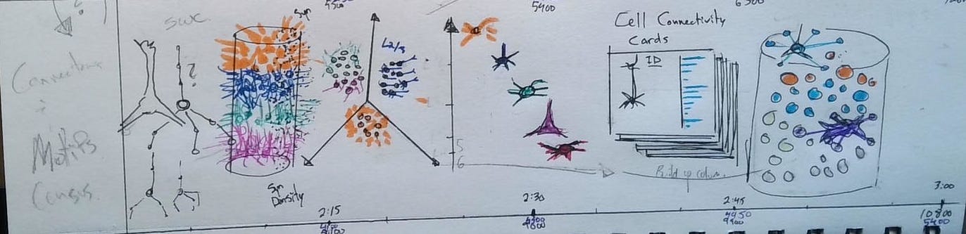
I found the “Compact cell connectivity cards” representation from Figure 6 of the paper to be an especially succinct and informative way of comparing the connectivity and morphology between cells. They quantitatively captured the magnitude and distribution of synaptic connectivity, while also highlighting the layer-spanning morphological features of the neurons.

An example cell connectivity card reproduction. I maintained the cell-type specific color palette, but I didn’t clean up the lines between dendritic segments as the left subplot was never going to have any screen time.

The challenge here was to recreate the cell cards in matplotlib, formatted such that it could be composited with the 3D renders in Blender. And the plots had to be aligned with the animation when played back at 60fps in the final video.

Video description:
We zoom into the same column of cortex, this time considering the entire neuron morphology. We see another low dimensional representation in UMAP space, this time the neuron morphology is shown for a selection of the points. The camera orbits and pans close to the cells so we can appreciate the structural differences between different types of neurons (referred to as “Morphological types”.

We then see one example inhibitory neuron, and slowly cycle through a visualization of its synapses onto the specific neuron types in the column. We start by seeing each layer's synapses individually from this single inhibitory neuron, then we show the connectivity for each of the inhibitory neurons in the study. This animated segment effectively recreates the ‘cell cards’ from the paper, but in animated form.

4. Foundation model of neural activity predicts response to new stimulus types

NeuroAI

Recall that what is extra special about this dataset is that the mouse watched videos while running on a treadmill and having a microscope connected to its brain, before its brain was digitized with electron microscopy. It’s a massive physiological experiment with a richness of data, and let them build a “Digital Twin’ of the cubic millimeter, trained on the neural responses to visual stimuli. Trained on actual neural responses, it can predict visual cortex response to new video not before seen in the training.

For this section, I wanted to borrow elements from the Figure 1’s from multiple papers in the package, and combine elements from both.

There was so much novelty in the technical approach in this paper, that all of my focus in the video went entirely there. This video took a different approach than the others, it was more of an animated schematic driven by real data. The video had to emphasize that the neurons were recording responding to a visual scene, an artificial neural network was built from the stimuli/responses, and could be used to test the networks response to new video. It’s a lot for under 60 seconds of video.

This one was challenging to conceptualize for me, but I wanted to show real neuron responses to visual stimuli, and juxtapose this with the ‘digital twin’ in silico neural responses. I also wanted to show the ‘hidden layers’ of the convolutional network.

The responses being shown of the neurons are the actual neuron responses to the video clip being shown. I liked the stormy brain cloud sitting in front of a TV, so I’m glad it made it all the way into the final version. The layers of the convolutional network were shown before being compressed into a ‘black box’.
Fun fact: I chose the ‘Berlin’ colormap because it’s a diverging colormap from blue to orange, with black in the middle, and it's only been added to matplotlib only recently, so is well-worth the update.

Video description:
Neural responses to visual stimuli are shown driving activity in 3D neuron meshes. As we orbit, the same stimuli are fed into an artificial neural network. A cascade of convolutional layers emerges, revealing feature maps matched frame-by-frame to the input video. Side-by-side, the “digital twin” forms: real neural responses drive cell meshes on the left, while simulated responses animate the “Digital Twin” on the right.

5. Functional connectomics reveals general wiring rule in mouse visual cortex

The mic-drop moment where form and function collide

This one deserves a history lesson. In 1949 in “The Organization of Behavior”, D.O Hebb wrote:

“When an axon of cell A is near enough to excite cell B and repeatedly or persistently takes part in firing it, some growth process or metabolic change takes place in one or both cells such that A's efficiency, as one of the cells firing B, is increased.”

Thereby immortalizing the concepts of Hebbian Learning and the Cell Assembly.

Did I mention my grandfather was a student of Donald Hebb at McGill? I tend to mention this in as many conversations as possible.

This mouthful was succinctly summarized by Carla Shatz in the timeless and more portable expression:

“Cells that fire together, wire together”.

Since this data has functional recordings and synaptic connectivity graphs for thousands of cells and an immortalized digital twin, this could be analyzed. From Figure 2, let’s call it the MICrONS addendum:

“Neurons with higher signal correlation are more likely to form synapses.”
[Over short and long distances]

So in this video I simply wanted to show that connected neuron fire more synchronously than unconnected ones.

From the paper, Figure 2 depicts an example cell and its short and long distance synapses. The plot shows the signal correlation, that I wanted to see in spikes.

To understand why this is visually challenging to convey, we must accept that therecan be some daylight between the polished and simplified takeaway message well-suited to a sound-bite or undergraduate lecture slide, like “Cells that fire together, wire together.”, and the more nuanced and subtle statistical relationships in actual science data. We’re used to seeing computer generated images of neurons firing in perfect synchrony, which expresses the distilled concept with no subtlety or ambiguity, great for conveying an idea. The brain is not so clean. In this animated segment I wanted to capture the real data as accurately as possible, while also highlighting the profundity I see in the message. This one takes some extra explanation:

The point of this video segment was to show that synaptically connected neurons fire more synchronously than unconnected ones, whether local connections or long distance connections.

Like in the paper, I broke down a selection of neurons into 4 groups:

1. Proximal, connected: Neurons that are located close to the reference neuron (inside V1) who are synaptically connected

2. Proximal, unconnected: An equivalently sized sample (to 1) of neurons located close to the reference neuron who are not synaptically connected.

3. Distal, connected: Neurons located in the neighboring brain region (HVA) which are synaptically connected to the reference neuron.

4. Distal, unconnected: An equivalently sized sample (to 3) of neurons in the neighboring area which are not synaptically connected to the reference neurons.

I used same deconvolved calcium trace was used in all four subplots as the reference. An equivalent number of sample neurons were chosen for both proximal and distal comparisons. The traces in the ‘previsualization’ plot above were color-mapped based on their correlation strength with the reference neuron, and their y offset in the plot ordered by the rank order of the correlation. I chose the magma colormap to be perceptually uniform, while also decreasing to black on the low end, to emphasize highlight correlated neuronal firing. I used the same colormap for the color of the spiking neurons in the video

tldr: You should see more bright flashing neurons in the connected neurons than the unconnected ones

Video description:
We end with a detailed case study: one reference neuron is shown flashing with its deconvolved spikes. Its synapses with nearby neurons are highlighted in orange. For all the spiking neurons, the warmth of the color color is proportional to the correlation of activity with the reference neuron. We first see the locally connected neurons, then a sample of the same number of locally unconnected neurons for comparison. We then show that the analysis was extended to long-distance connections by showing synapses that the reference neuron makes with neurons in a neighboring cortical region (HVA = Higher Visual Areas). We first see the deconvolved spikes from the long distance connected neurons, followed by the long distance unconnected ones.

Even with the visual elements adapted in favor of showing the effect, it can still be subtle and difficult to pick out by the eye what are ultimately statistical relationships between a bunch of flashing lights. I guess this is why the raster plot is still so popular, and perhaps another good avenue to explore data sonification of spike data in the future.

Conclusion

For me, making a science video isn’t being a data clip from a scientist and then explaining it. It’s an in-depth journey into the paper, where I try to read it as an expert and an outsider simultaneously. From that unique vantage point I then take a deep dive into the data, often having to do my own analytical programming on the side, and always visual prototyping before I can even think about 3D models. While this article has described a specific project from preprint to postproduction, I only scratch the surface on other aspects of my workflow that I may explore further in future posts.

As they say in the business: don’t forget to smash that subscribe button, and until next time you can find me at Quorumetrix Studio on Bluesky, X, LinkedIn, and YouTube.